Introduction to Spectral Smoothing using the Radiometric Processing System in Oasis montaj

The Radiometric Processing System (RPS) is available for the first time with the 2025.2 release of Oasis montaj. It has been developed in partnership with Medusa Radiometrics, to provide a comprehensive processing workflow, for modern 1024-channel airborne gamma-ray spectrometers. It replaces our older 256-channel and Praga4 radiometric extensions.
A significant part of the RPS is a modern implementation of spectral smoothing, using Noise Adjusted Singular Value Decomposition (NASVD), which is a widely accepted type of Principal Component Analysis that is employed to smooth gamma-ray spectra prior to generating and processing radioelement counts. Here is a brief introduction to the technique, why it is used and how it is implemented in Oasis montaj.
Why is NASVD Necessary?
Gamma-ray spectrometer data is inherently noisy. This is because radioactive decay is a random, statistical process. This randomness, combined with the low number of gamma rays detected per second, results in a low signal-to-noise ratio.
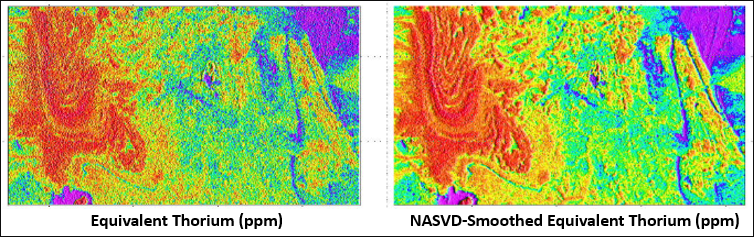
As with almost all geophysical methods, improving the signal-to-noise ratio makes the final data much easier to interpret geology or otherwise from; the example below compares a thorium count with one that has been smoothed using NASVD:
How does NASVD Work?
NASVD works by decomposing the variations in the spectral data into a series of fundamental spectral "shapes," called principal components. The first few components represent the most significant and coherent signals in the data—primarily the characteristic spectra of Potassium, Uranium, and Thorium. The remaining, higher-order components represent the random, non-coherent noise.
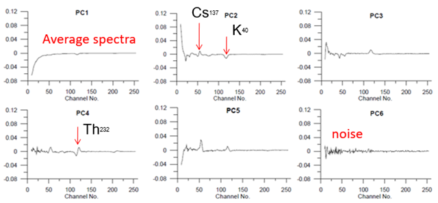
This graphic shows the first six principal components of a typical (256-channel in this case) gamma-ray spectrum (adapted from Mauring & Smethurst, 2005). The first component (PC1) represents the average spectra. Components 2-5 show a signal at channel 55 from Caesium-137 and the channels 109-125 show a signal from Potassium-40. In this case, the components are shifted slightly due to instrument drift. Component 4 shows a signal from Thorium-232 between channels 189-220. Component 6 is dominated by noise, so in this case five components are likely enough to reconstruct the signal, using NASVD.
Reconstructing the original spectrum using only these first few "signal" components, from a much larger set (typically 10-20) of components, results in a spectrum that retains the essential information while eliminating most of the noise.
Applying NASVD in the Radiometric Processing System
A key to using NASVD is identifying how many principal components, or eigenvector, to use when reconstructing the spectrum. There is not a lot of consensus among experts or established "best practice" with respect to this, other than agreement that careful analysis of the eigenvectors and their associated eigenvalues is required. We designed the Smooth Spectra dialog to make this analysis as straightforward as possible. A typical application of NASVD in Oasis montaj involves the following steps:
1: Define the input energy range
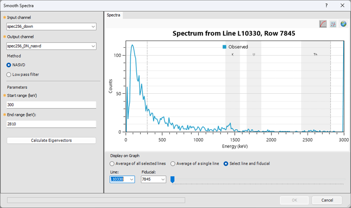
Limiting the input energy range is a common means of improving the signal to noise ratio prior to performing NASVD. We can do this because:
- the very low (<300 keV) energy channels often have high noise levels and significant interference from the detector system itself and other non-geological background sources
- above 3000 keV, count rates for natural sources are very low, and the signal is dominated by high-energy cosmic rays, which typically traverse the detector without full interaction and do not contribute useful spectral shapes for the analysis of natural radioelements
- the NASVD method assumes a Poisson noise distribution and exploits the high correlation between different channels in the signal component. Limiting the data to the range where the signal is strong and correlated ensures these assumptions are met, leading to more robust results.
2: Calculate and select the number of eigenvectors to use
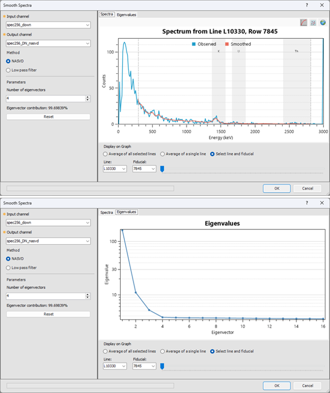
Once the eigenvectors are calculated, the Smooth Spectra plot updates to (a) show a preview of the smoothed spectra (orange line) and (b) shows a plot of the eigenvalues for each eigenvector. This plot shows the eigenvectors (which represent the directions of maximum variance), plotted against their corresponding eigenvalues (which indicates the amount of variance). Note also the reported Eigenvector contribution in the left pane; this shows the percentage of the original data that will be preserved within the reconstructed (smoothed) spectra, for the corresponding number of eigenvectors.
With respect to choosing an appropriate number of eigenvectors to use, we recommend identifying the inflection point where the eigenvalue curve begins to flatten to a straight line; in the example above, this occurs at eigenvector 4. If we were to choose to use these 4 eigenvectors when applying NASVD, ~99.7% of the input spectrum will be retained in the smoothed output.
An e-learning course that covers the full use of the Radiometrics Processing System in Oasis montaj will be released in late February..
Reference:
Mauring, E., & Smethurst, M. A. (2005). Reducing noise in radiometric multi-channel data using noise-adjusted singular value decomposition (NASVD) and maximum noise fraction (MNF). NGU-RAPPORT, 2005.014.