GM-SYS 3D - Synthetic Sensitivity Modelling Study

MartinVogele

Good morning all,

I am currently running simplified 3D wedge models approximating my geological scenario with the ultimate goal to assess resulting depthing uncertainties through structural Inversion considering the inherent input density and picking uncertainties.


After running some initial tests, I discovered some modelling inconsistencies which I tried to understand by furtehr simplifying my 3D model:

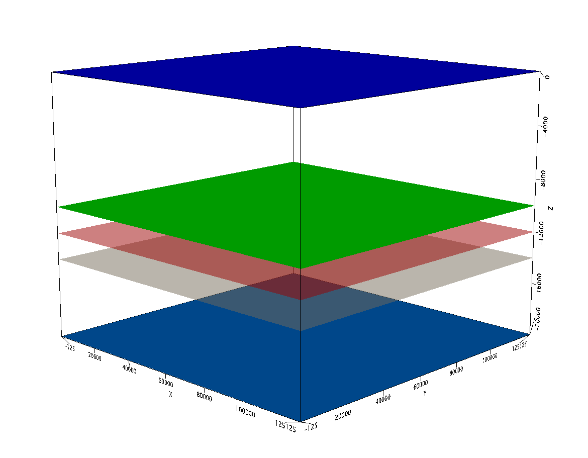
1) Assuming a two-layered rectangular model (see screenshot 1), with rho1 in the upper layer, seperated by the red surface at Z1 from rho2 and the lower layer, producing my reference case (GOBS). (The green and gray surfaces are not used here and solely indicate the position of the red surface in the subsequent experiments.)

2) Secondly, I ran two scenarios where the red surface was shifted up (green surface Z2 < Z1) and down (gray surface Z3 > Z1) producing two different uniform gravity grids GCALC2 and GCALC3. DC-shift was set to zero.

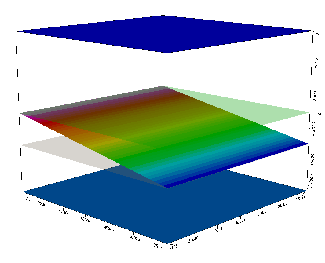
3) Thirdly, I ran a scenario, where the red surface was tilted (screenshot 2) with the minimum depth being equal to the previously used green surface and the maximum depth being equal to the gray surface (Z2 <= Z4 <= Z3). I then ran the model again to produce a third anomaly grid GCALC4.




>> When I now compare the obtained gravity anomalies GCALC2, -3, and -4 with GOBS, I realised that the maximum and minimum of GOBS4 (wedge model) were not equal to GCALC2 and GCALC3 from the planar models 2 (green surface) and 3 (gray surface) despite having the same maximum and minimum depths at the model boundaries of the green and gray surface...

- Is this related to the fact that Geosoft does not only calculate the vertical attraction of the model but also takes into consideration lateral density heterogenities? If yes, up to which distance?

- Generally speaking, do you think it is worth to run sensitivity models of simplified geological scenarios (average depth of surfaces, gradually variying densities) to quantify depthing uncertainties, i.e. through structural Inversion, taking into account inherent uncertainties of input data?


Many thanks in advance for your support and best regards,

Martin


Screenshot 1


Screenshot 2

GerryConnard

Martin,

Flat, constant thickness, constant density, infinite (in X & Y) layers produce a flat response. You can calculate the response using the Bouguer slab formula (2*pi*G*rho*h). Most gravity measurements are relative measurements so flat models are not particularly useful for real world problems.

The vertical attraction at any measurement point is strongly impacted by lateral density heterogeneities, in theory, out to "infinity". The magnitude of course depends on the size, shape, and density of the lateral density heterogeneities. For example, the vertical attraction of a sphere = Gmz/(r*r*r) where G is the gravity constant, m is the mass of the sphere, z is the depth of the sphere, and r is the radial distance from the measurement point to the center of the sphere.

In our space-domain calculations, we extend the models out to 50,000 km to minimize this effect. GM-SYS 3D mainly uses frequency-domain (FFT) calculations which assume that the model is repeated in all directions out to infinity. The model you see is smoothly expanded and made periodic to minimize "edge effects" by the calculation routine. The default expansion factor is 50% but the user can set that factor. The expansion factor affects the calculation time.

Generally speaking, I think it is quite useful to run sensitivity models to quantify all sorts of uncertainties including depth uncertainties. I recommend this for designing gravity surveys.